▶️ Watch on 3Speak - Odysee - BitChute - Rumble - YouTube - PDF Notes - Summary - Sections playlist - Vector Functions playlist

---

In this video I deep dive nearly 5 hours into vector functions and space curves. A vector function has a domain (or input) of real numbers and a range (or outputs) of vectors. Compare this with the real-valued functions that we are used to, which have inputs of real numbers (typically x) and the outputs are also real numbers (typically y = f(x)).

Vector functions can be written as there component parts, which are made up of real-valued functions. In this chapter I focus on vector functions with 3 component parts because they can be plotted in three dimensional parts. Obtaining the parametric equations of such vector functions obtains a space curve. That is, a curve that can be plotted in 3D space. I also dive into the limits of vector functions, and show how to plot space curves with 3D graphing calculators such as GeoGebra. Buckle up!

Timestamps

• Introduction: 0:00
• Calculus Book Reference: 0:48
• Calculus Book Chapter: 1:08
• Topics to Cover: 1:40
• Vector Functions: 2:37
• Vector Functions and Space Curves: 4:04
  • Example 1: 8:03
• Limit of a Vector Function: Definition 1: 13:08
  • Example 2: 17:04
• Space Curves: 23:33
  • Example 3: 29:07
• Plane Curves: 33:15
  • Example 4: 36:00
  • DNA Helix: 44:03
• Example 5: 48:10
• Example 6: 1:00:20
• Using Computers to Draw Space Curves: 1:19:21
  • Example 7: Twisted Cubic: 1:22:37
  • Visualizing Space Curves on Surfaces: 1:27:59
• Charged Particle Moving in an Electromagnetic Field: 1:32:40
  • The Physics of Charged Particles in Electromagnetic Fields: 1:44:32
• Exercises
• Exercise 1: Precise Definition of a Vector Function Limit: 2:14:20
  • Recap on Real-Valued Function Limits: 2:15:48
  • Solution 1: 2:19:40
  • Solution 2: 2:36:54
  • Visualizing the Precise Definition of a Vector Function Limit: 2:46:14
• Exercise 2: Properties of Vector Function Limits: 2:54:25
  • Solution: 2:55:44
  • Solution to (a): 2:57:03
  • Solution to (b): Constant multiple limit: 3:06:21
  • Solution to (c): Dot Product limit: 3:10:35
  • Solution to (d): Cross Product limit: 3:17:11
• Exercise 3: Trefoil Knot: 3:28:51
• Exercise 4: Trochoid: 4:21:00
• Outro: 4:45:23

---

View Video Notes Below!

---

Become a MES Super Fan - Donate - Subscribe via email - MES merchandise

• MES Links webpage - MES Links Telegram - MES Truth

Reuse of my videos:

• Feel free to make use of / re-upload / monetize my videos as long as you provide a link to the original video.

Fight back against censorship:

• Bookmark sites/channels/accounts and check periodically.
• Remember to always archive website pages in case they get deleted/changed.

Recommended Books: "Where Did the Towers Go?" by Dr. Judy Wood

Join my forums: Hive community - Reddit - Discord

Follow along my epic video series: MES Science - MES Experiments - Anti-Gravity (MES Duality) - Free Energy - PG

---

NOTE 1: If you don't have time to watch this whole video:

• Skip to the end for Summary and Conclusions (if available)
• Play this video at a faster speed.
  -- TOP SECRET LIFE HACK: Your brain gets used to faster speed!
  -- MES tutorial
• Download and read video notes.
• Read notes on the Hive blockchain $HIVE
• Watch the video in parts.
  -- Timestamps of all parts are in the description.

Browser extension recommendations: Increase video speed - Increase video audio - Text to speech (Android app) – Archive webpages

---

Calculus Book Reference

Note that I mainly follow along the book:

• Calculus: Early Transcendentals 7th Edition by James Stewart: Link
  • I used the following solution manual for this chapter: Link
• Note: In some earlier videos I used the 6th edition.

---

Calculus Book Chapter

The Hive notes and sections playlist for each video of this chapter are listed below:

Vector Functions ▶️

1. Vector Functions and Space Curves - ▶️
2. Derivatives and Integrals of Vector Functions
3. Arc Length and Curvature
4. Motion in Space: Velocity and Acceleration
   • Applied Project: Kepler's Laws
5. Review
   • Concept Check
   • True-False Quiz
6. Problems Plus

This links are also on MES Links: https://mes.fm/links

---

Topics to Cover

Note that the timestamps will be included in the video description for each topic listed below.

• Vector Functions
• Vector Functions and Space Curves
  • Example 1
• Limit of a Vector Function: Definition 1
  • Example 2
• Space Curves
  • Example 3
• Plane Curves
  • Example 4
  • DNA Helix
• Example 5
• Example 6
• Using Computers to Draw Space Curves
  • Example 7: Twisted Cubic
  • Visualizing Space Curves on Surfaces
• Charged Particle Moving in an Electromagnetic Field
  • The Physics of Charged Particles in Electromagnetic Fields
• Exercises
• Exercise 1: Precise Definition of a Vector Function Limit
  • Recap on Real-Valued Function Limits
  • Solution 1
  • Solution 2
  • Visualizing the Precise Definition of a Vector Function Limit
• Exercise 2: Properties of Vector Function Limits
• Exercise 3: Trefoil Knot
• Exercise 4: Trochoid

---

Vector Functions

The functions that we have been using so far have been real-valued functions.

We now study functions whose values are vectors because such functions are needed to describe curves and surfaces in space.

We will also use vector-valued functions to describe the motion of objects through space.

In particular, we will use them to derive Kepler's laws of planetary motion.

Kepler's First Law says that the planets revolve around the sun in elliptical orbits.

In a later video, we will see how the material of this chapter is used in one of the great achievements of calculus: proving Kepler's Laws.

---

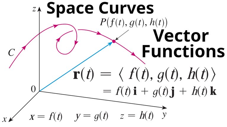
Vector Functions and Space Curves

In general, a function is a rule that assigns to each element in the domain an element in the range.

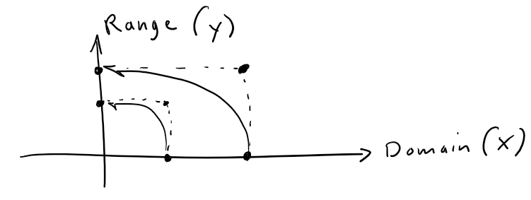
A vector-valued function, or vector function, is simply a function whose domain is a set of real numbers and whose range is a set of vectors.

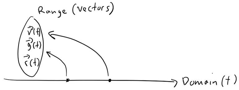
We are most interested in vector functions r whose values are three-dimensional vectors.

This means that for every number t in the domain r there is a unique vector in V3 denoted by r(t).

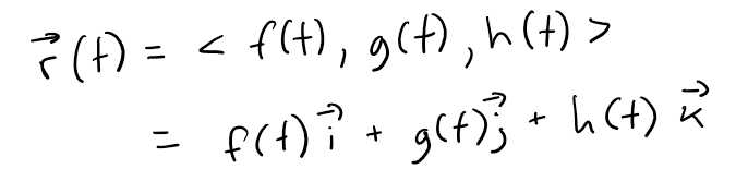
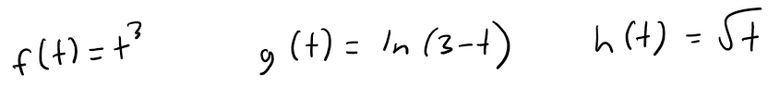
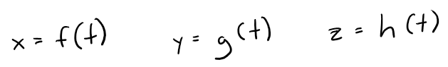
If f(t), g(t), and h(t) are the components of the vector r(t), then f, g, and h are real-valued functions called the component functions of r and we write:

We use the letter t to denote the independent variable because it represents time in most applications of vector functions.

---

Example 1

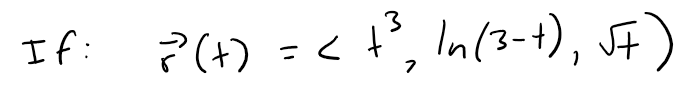
then the component functions are:

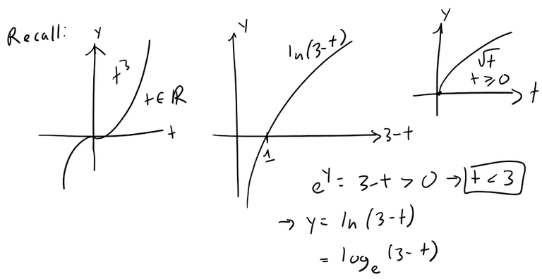
By our usual convention, the domain of r consists of all values of t for which the expression for r(t) is defined.

The expressions t³, ln(3-t), and t^1/2 are all defined when 3 - t > 0 and t ≥ 0.

Therefore the domain of r is the interval [0, 3).

---

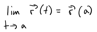
Limit of a Vector Function

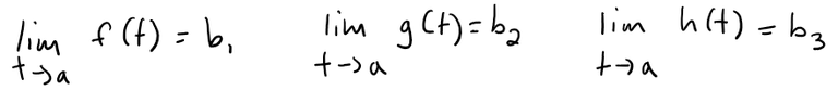
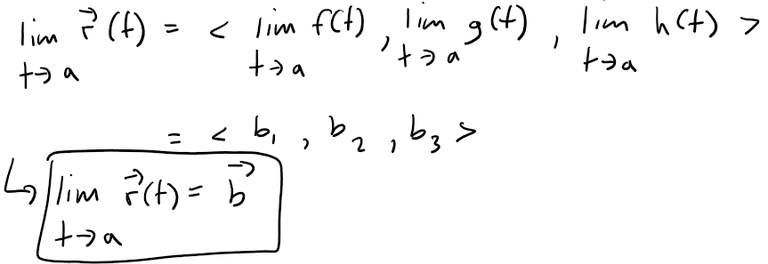
The limit of a vector function r is defined by taking the limits of its component functions as follows.

Definition 1

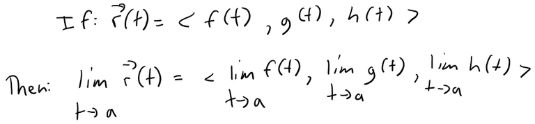
Provided the limits of the component functions exist.

Note: If lim_t→ar(t) = L, this definition is equivalent to saying that the length and direction of the vector r(t) approach the length and direction of the vector L.

Equivalently, we could have used an ε-δ definition (see Exercise 1).

Limits of vector functions obey the same rules as limits of real-valued functions (see Exercise 2).

---

Example 2

Find lim_t→0r(t), where:

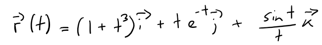
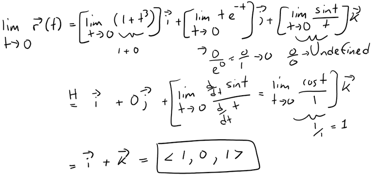
Solution:

According to Definition 1, the limit of r is the vector whose components are the limits of the component functions of r:

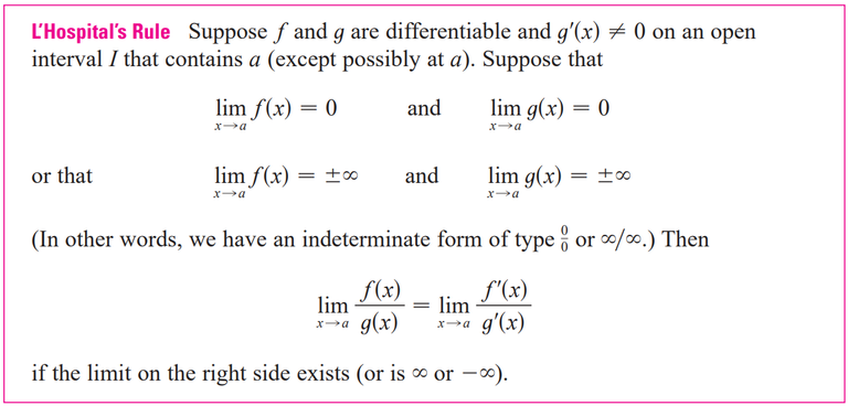
Recap on L'Hospital's Rule from my earlier video:

---

Space Curves

A vector function r is continuous at a if:

In view of Definition 1, we see that r is continuous at a if and only if its component functions f, g, and h are continuous at a.

There is a close connection between continuous vector functions and space curves.

Suppose that f, g, and h are continuous real-valued functions on an interval I.

Then the set C of all points (x, y, z) in space, where:

and t varies through the interval I, is called a space curve.

The equations above are called parametric equations of C and t is called a parameter.

We can think of C as being traced out by a moving particle whose position at time t is ( f(t), g(t), h(t) ).

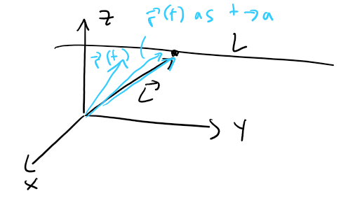
If we now consider the vector function r(t) = < f(t), g(t), h(t) >, then r(t) is the position vector of the point P( f(t), g(t), h(t) ) on C.

Thus any continuous vector function r defines a space curve C that is traced out by the tip of a moving vector r(t), as shown in the figure below.

C is traced out by the tip of a moving position vector r(t).

---

Example 3

Describe the curve defined by the vector function:

r(t) = < 1 + t, 2 + 5t, -1 + 6t >

Solution:

The corresponding parametric equations are:

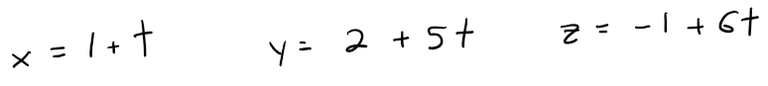
which we recognize from my earlier video as parametric equations of a line passing through the point (1, 2, -1) and parallel to the vector <1, 5, 6>.

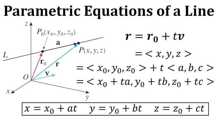
Alternatively, we could observe that the function can be written as r = r₀ + tv, where r₀ = <1, 2, -1> and v = <1, 5, 6>, and this is the vector equation of a line as given by the above image and my other earlier video.

---

Plane Curves

Plane curves can be also be represented in vector notation.

For instance, the curve given by the parametric equations x = t² - 2t and y = t + 1 (see my earlier video could also be described by the vector equation:

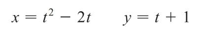
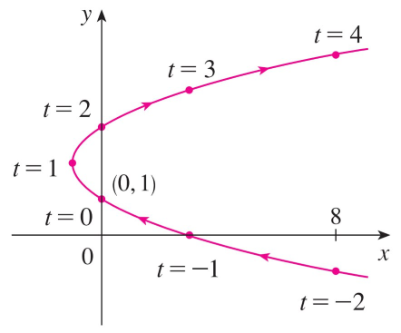
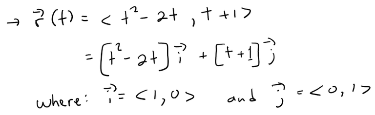
Recall from my earlier video that i, j, and k are standard basis vectors in 3D.

---

Example 4

Sketch the curve whose vector equation is:

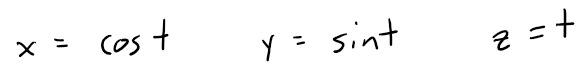
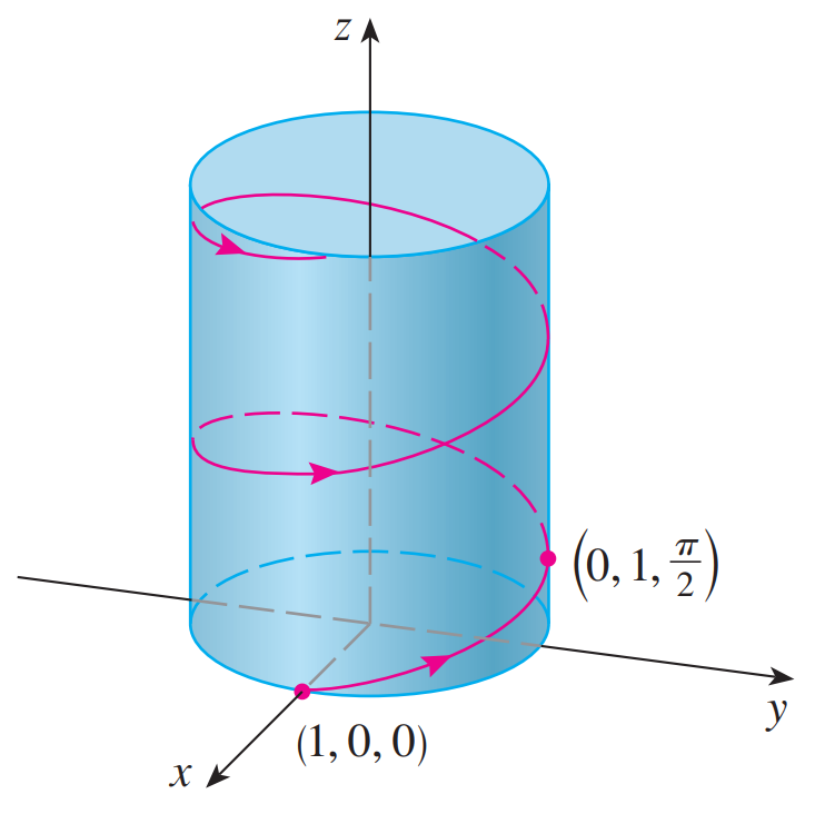
r(t) = cos t i + sin t j + t k

Solution:

The parametric equations for this curve are:

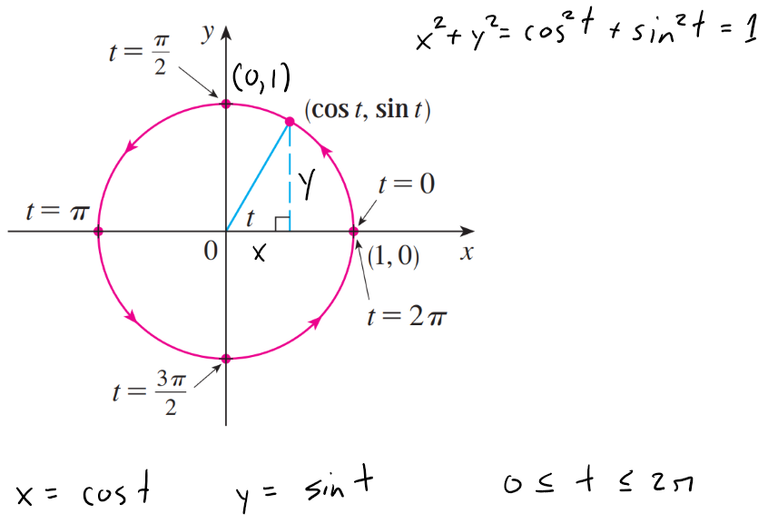
Since:

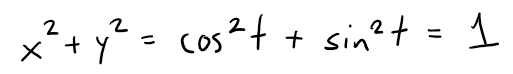
Then the curve must lie on the circular cylinder x² + y² = 1.

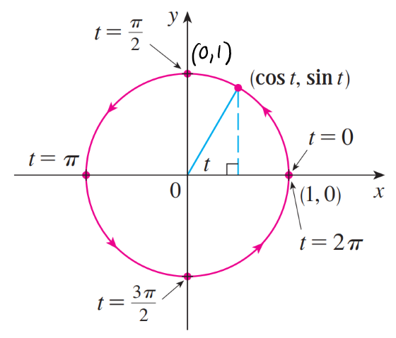
The point (x, y, z) lies directly above the point (x, y, 0), which moves counterclockwise around the circle x² + y² = 1 in the xy-plane.

The projection of the curve onto the xy-plane has vector equation:

r(t) = <cos t, sin t, 0>

See my earlier video.

Since z = t, the curve spirals upward around the cylinder as t increases.

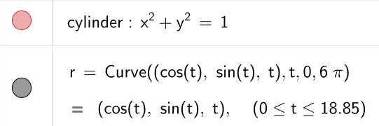
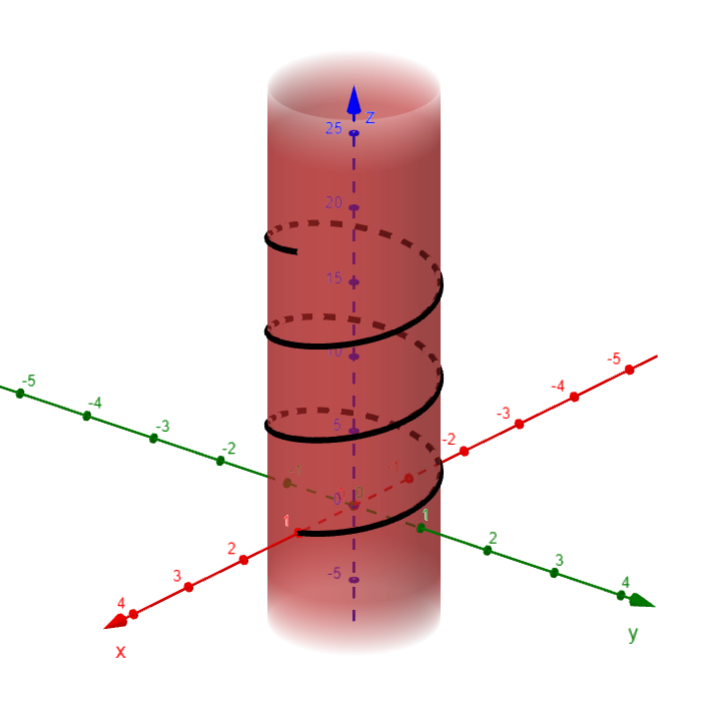
The curve, shown in the figure below, is called a helix.

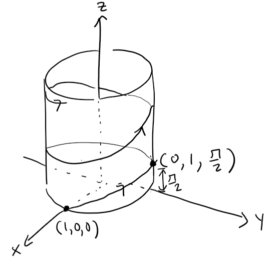
Here is a better illustration from my calculus book.

Here is the graph in GeoGebra's 3D graphing calculator.

[https://www.geogebra.org/3d/ukqwffru]https://www.geogebra.org/3d/ukqwffru)

---

DNA Helix

The corkscrew shape in Example 4 is familiar from its occurrence in coiled springs.

It also occurs in the model of DNA (deoxyribonucleic acid, the genetical material of living cells).

In 1953 James Watson and Francis Crick showed that the structure of the DNA molecule is that of two linked, parallel helixes that are intertwined as in the figure below.

A double helix

Here is more info on DNA and RNA from my earlier videos.

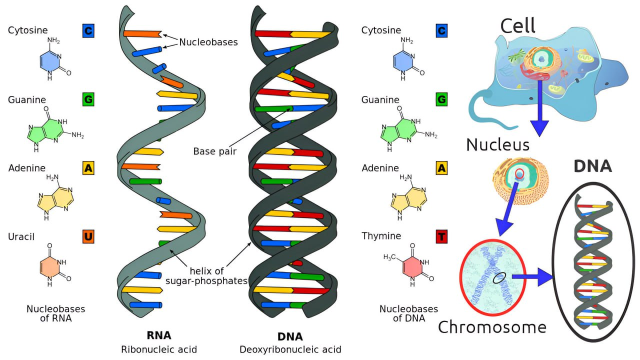
DNA is contained in the nucleus every cell of the body.

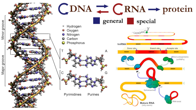
Central dogma of molecular biology states that information flows from DNA to/from RNA to protein and never from protein.

---

Example 5

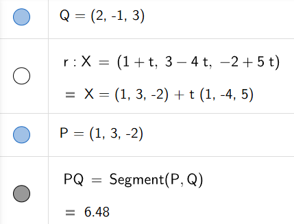
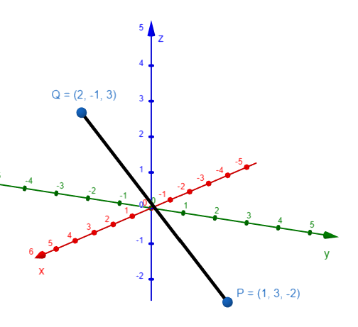
Find a vector equation and parametric equations for the line segment that joins P(1, 3, -2) to the point Q(2, -1, 3).

Solution:

In my earlier video, we found a vector equation for the line segment that joins the tip of the vector r₀ to the tip of the vector r₁:

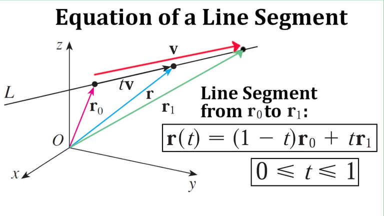
In our case, the vector equation of the line segment from P to Q is:

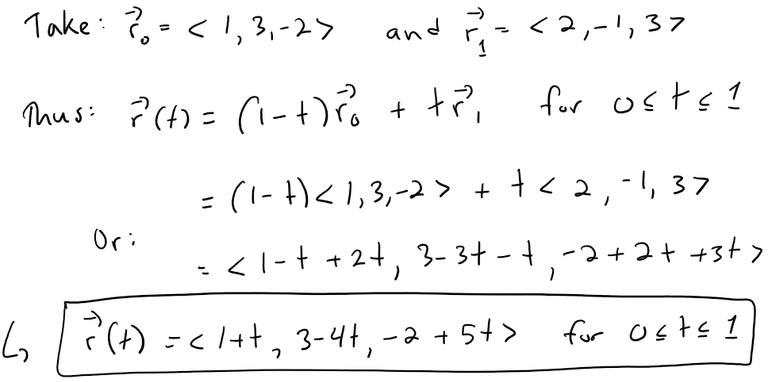
The corresponding parametric equations are:

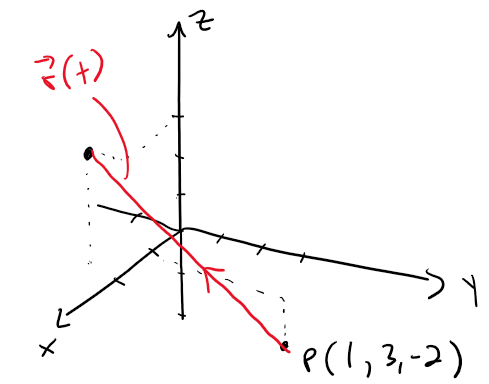
The line segment PQ is graphed below.

Here is the graph in GeoGebra's 3D graphing calculator.

https://www.geogebra.org/calculator/uh9jnevt

---

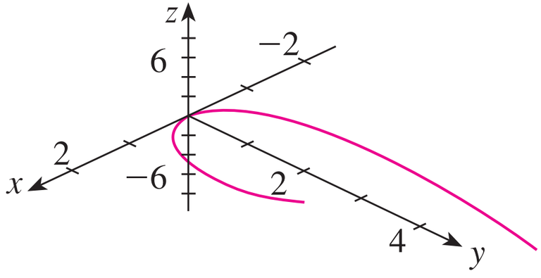
Example 6

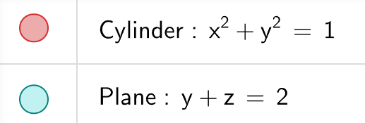
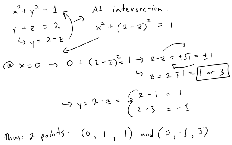
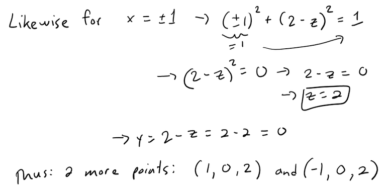
Find a vector that represents the curve of intersection of the cylinder x² + y² = 1 and the plane y + z = 2.

Solution:

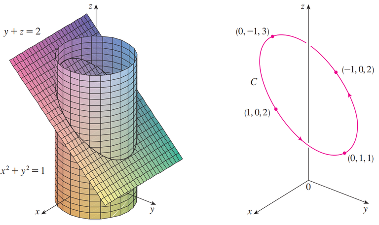
The figure below shows how the plane and the cylinder intersect.

https://www.geogebra.org/calculator/v7ecchdb

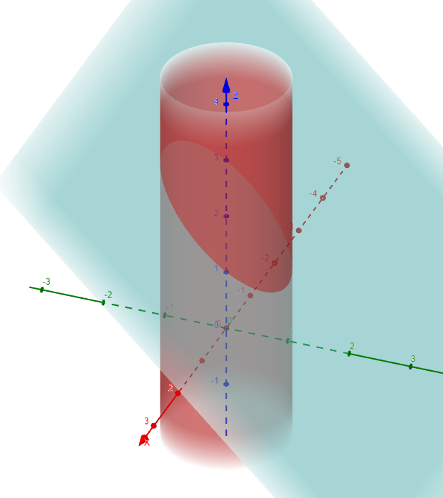
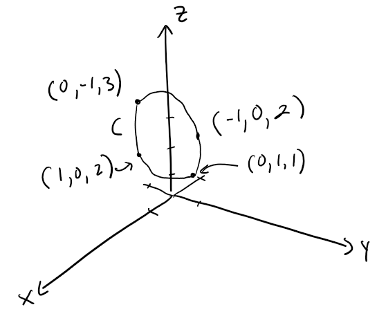
The figure below shows the curve of intersection C, which is an ellipse.

Here is a better illustration from my calculus book.

The projection of C onto the xy-plane is the circle x² + y² = 1, z = 0.

So we know from my earlier video that we can write:

From the equation of the plane, we have:

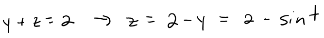
So we can write parametric equations for C as:

The corresponding vector equation is:

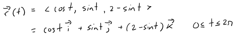
This equation is called a parametrization of the curve C.

The arrows in the earlier figure indicate the direction in which C is traced as the parameter t increases.

---

Using Computers to Draw Space Curves

Space curves are inherently more difficult to draw by hand than plane curves; for an accurate representation we need to use technology.

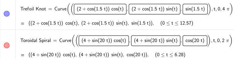
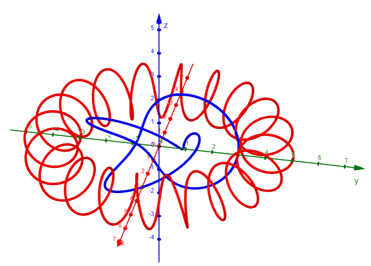
For instance, the figure below shows a computer generated graph of the curve with parametric equations:

x = (4 + sin 20t) cos t
y = (4 + sin 20t) sin t
z = cos 20t

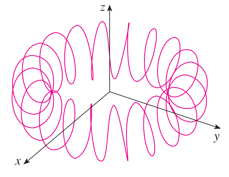
A toroidal spiral

It's called a toroidal spiral because it lies on a torus.

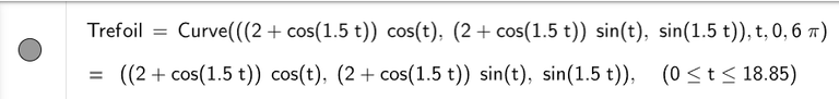
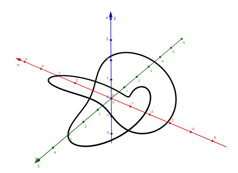
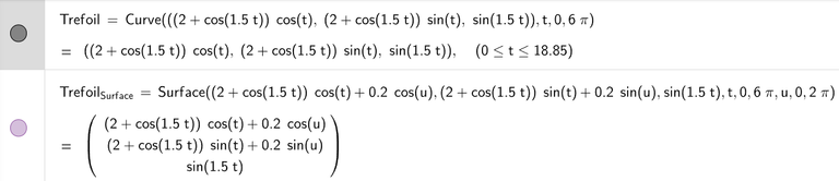
Another interesting curve, the trefoil knot, with equations:

x = (2 + cos 1.5t) cos t
y = (2 + cos 1.5t) sin t
z = sin 1.5t

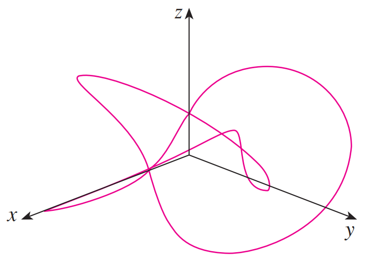
A trefoil knot

Here are the graphs in GeoGebra:

https://www.geogebra.org/calculator/gyfv87f2

Even when a computer is used to draw a space curve, optical illusions make it difficult to get a good impression of what the curve really looks like.

This is especially true in the trefoil knot above (see Exercise 3).

The next example shows how to cope with this problem.

---

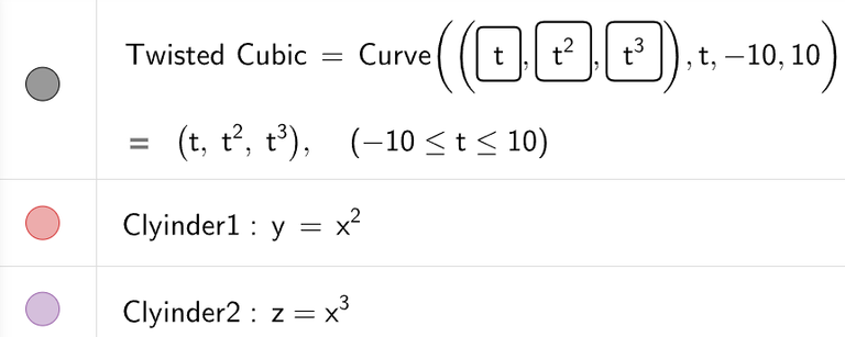
Example 7: Twisted Cubic

Use a computer to draw the curve with vector equation r(t) = <t, t², t³>.

This curve is a called a twisted cubic.

Solution:

We start by using the computer to plot the curves with parametric equations:

x = t, y = t², z = t³ for - 2 ≤ t ≤ 2.

The result is shown in the figure below, but it's hard to see the true nature of the curve from the graph alone.

Most three-dimensional computer graphing programs allow the user to enclose a curve or surface in a box instead of displaying the coordinate axes.

When we look at the same curve in a box, as in the figure below, we have a much clearer picture of the curve.

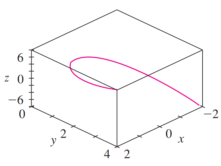
We can see that it climbs from a lower corner of the box to the upper corner nearest us, and it twists as it climbs.

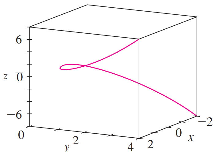
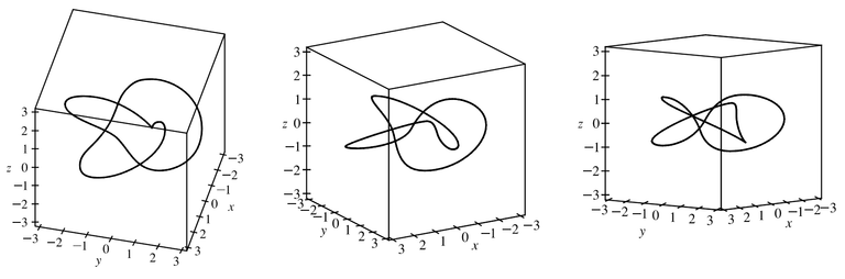
We can get an even better idea of the curve when we view it from different vantage points.

The figure below shows the result of rotating the box to give another viewpoint.

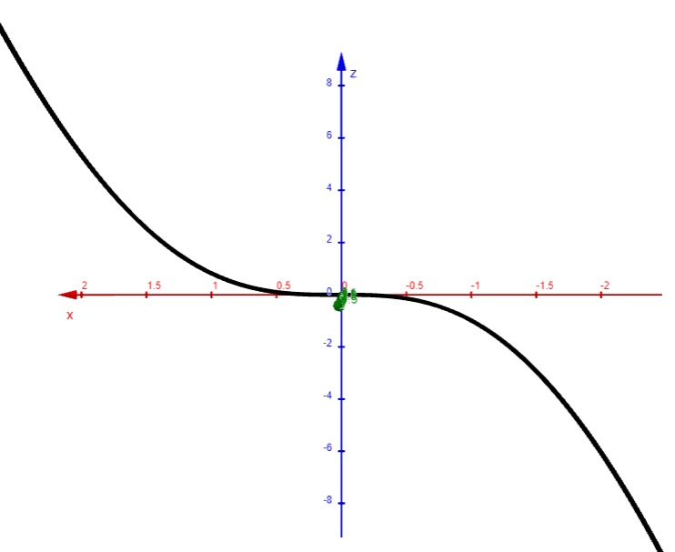
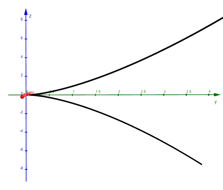
The figures below shows the views we get when we look directly at a face of the box.

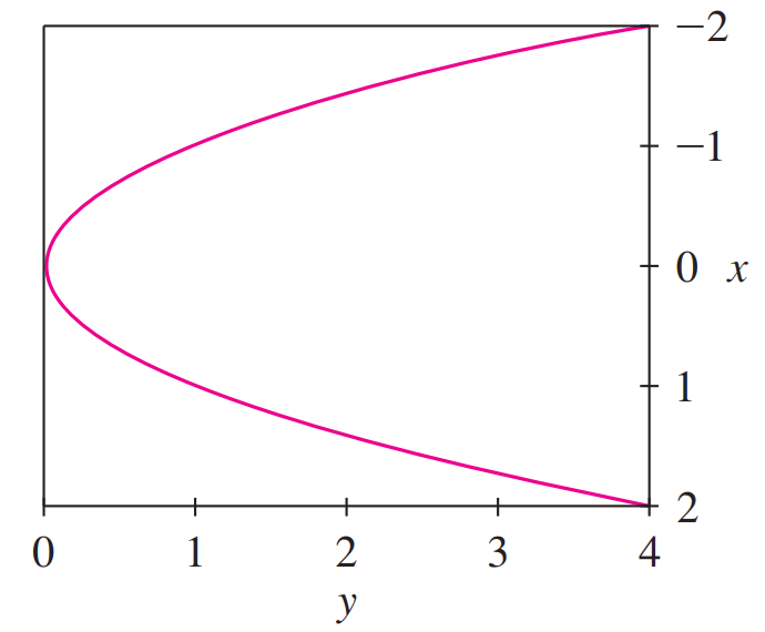
Top view

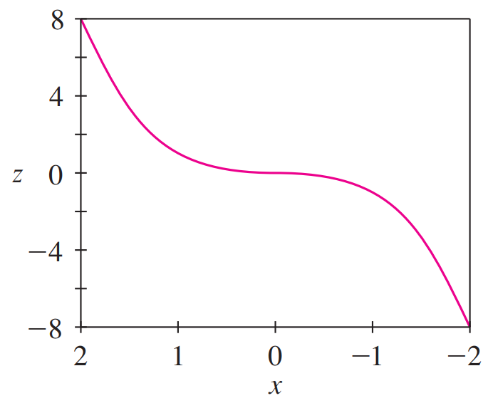
Side view

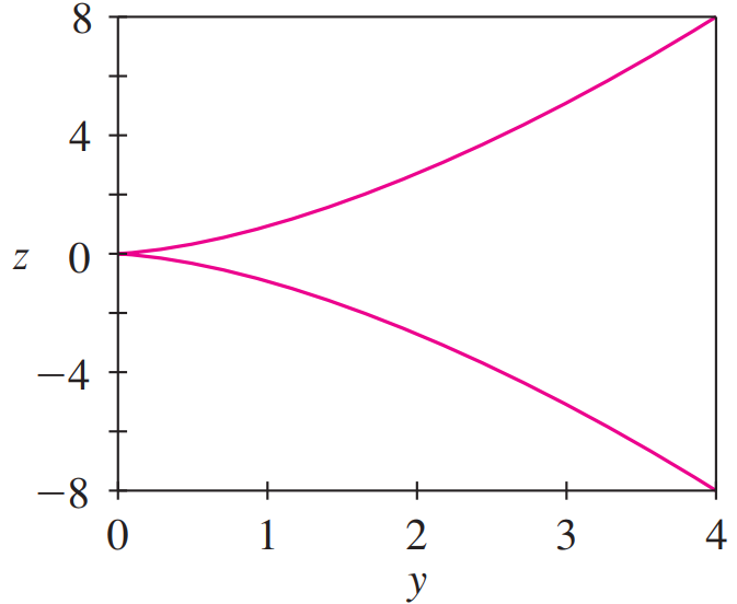
Front view

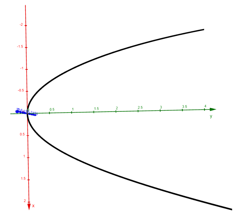
In particular, the top view shows the view from directly above the box.

It is the projection of the curve on the xy-plane, namely, the parabola y = x².

The side view shows the projection on the xz-plane, the cubic curve z = x³.

It's now obvious why the given curve is called a twisted cubic.

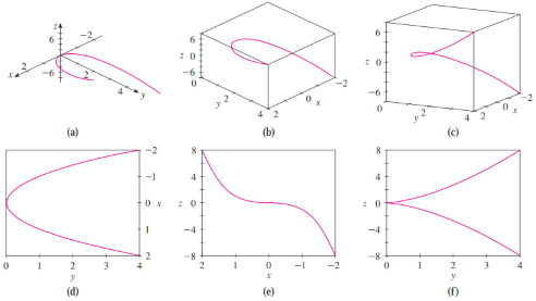
Views of the twisted cubic

Here is the graph in GeoGebra.

https://www.geogebra.org/calculator/vxv5heat

---

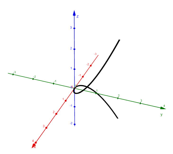
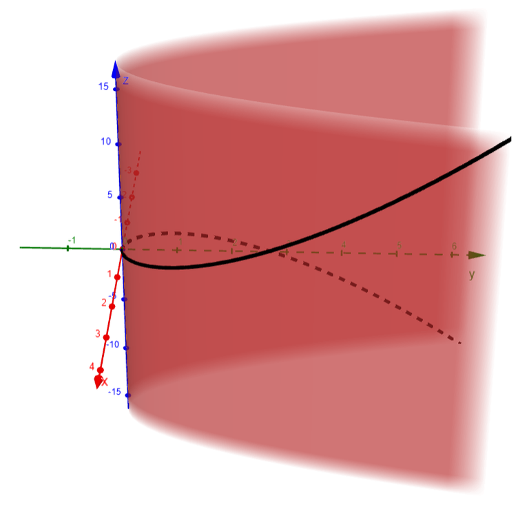
Visualizing Space Curves on Surfaces

Another method of visualizing a space curve is to draw it on a surface.

For instance, the twisted cubic in Example 7 lies on the parabolic cylinder y = x².

We can see this when we eliminate the parameter t from the first two parametric equations, x = t and y = t².

The figure below shows the cylinder and the twisted cubic, and we see that the curve moves upward from the origin along the surface of the cylinder.

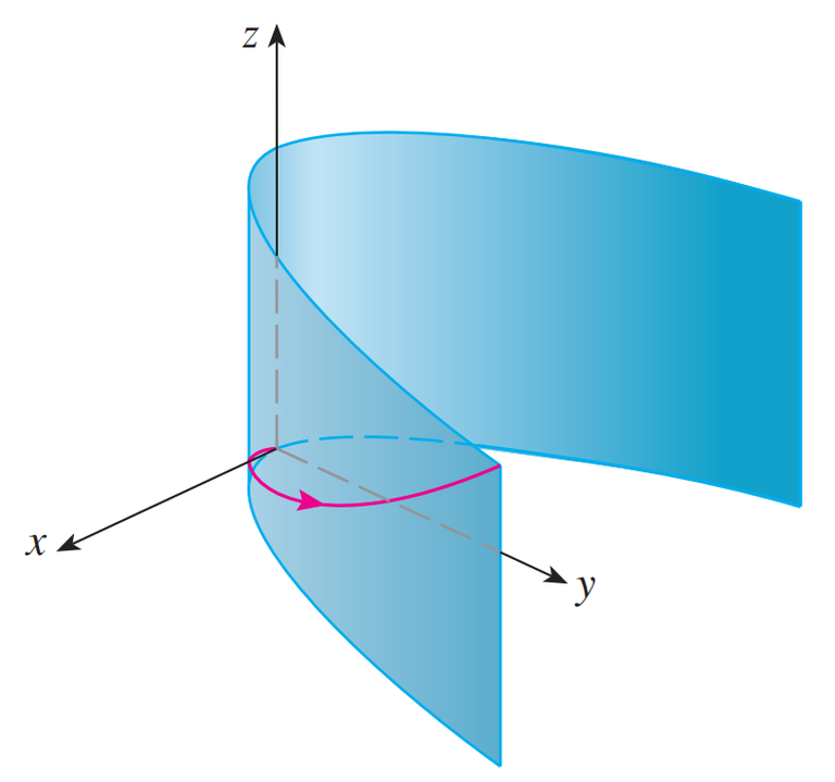
We also used this method in Example 4 to visualize the helix lying on the circular cylinder.

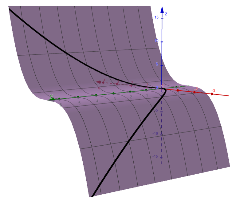
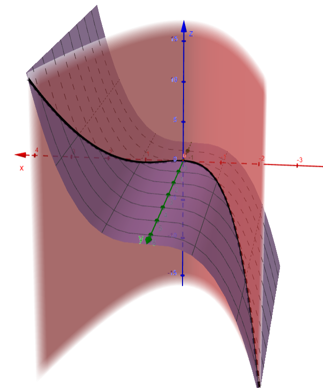
A third method for visualizing the twisted cubic is to realize that it also lies on the cylinder z = x³.

So it can be viewed as the curve of intersection of the cylinders y = x² and z = x³, as in the figure below.

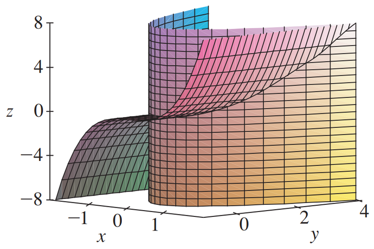
Let's graph this in GeoGebra.

https://www.geogebra.org/calculator/vxv5heat

---

Charged Particle Moving in an Electromagnetic Field

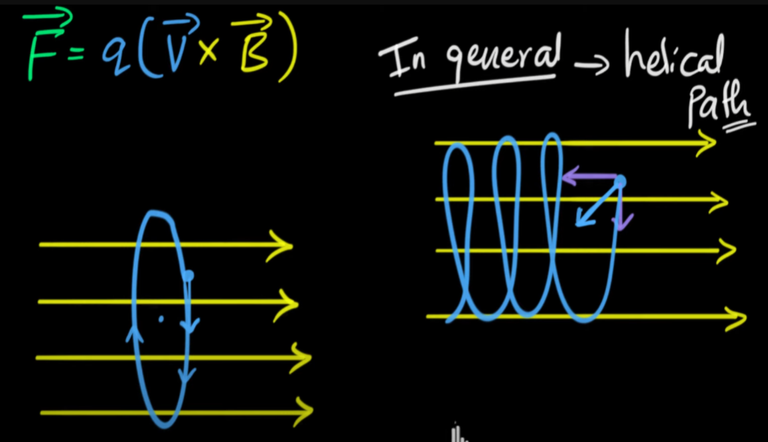
We have seen that an interesting space curve, the helix, occurs in the model of DNA.

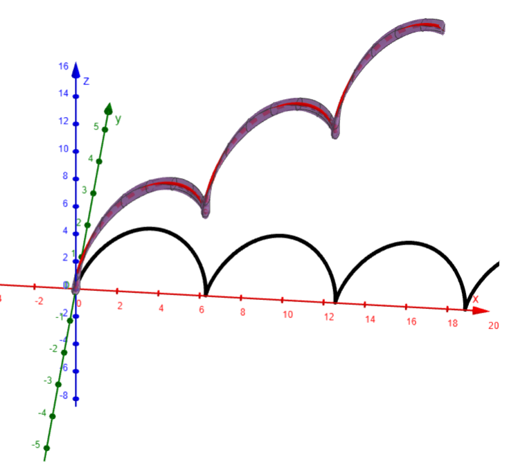
Another notable example of a space curve in science is the trajectory of a positively charged particle in orthogonally oriented electric and magnetic fields E and B.

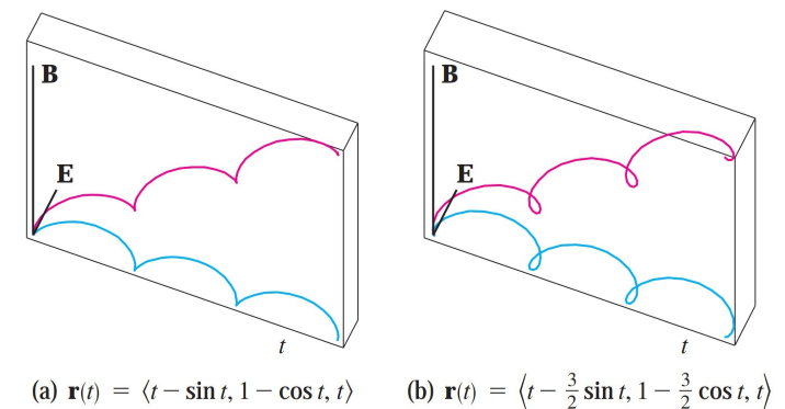
Motion of a charged particle in orthogonally oriented electric and magnetic fields

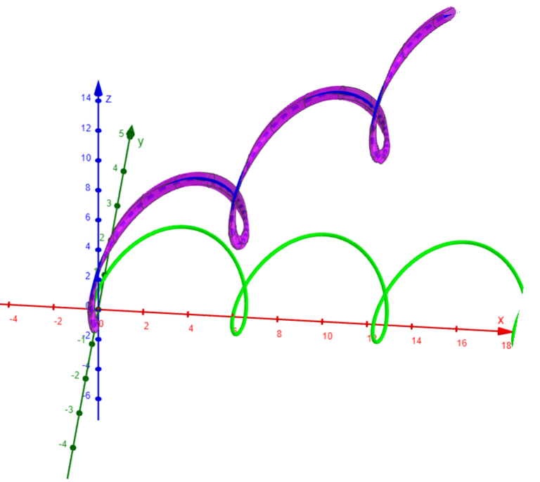
Depending on the initial velocity given the particle at the origin, the path of the particle is either (a) a space curve whose projection on the horizontal plane is the cycloid we studied in my earlier video or (b) a curve whose projection is the trochoid (see Exercise 4).

The cycloid is formed by tracing the position of a point on a circle as it rolls.

The trochoid is formed by tracing any point inside, on (hence a cycloid), or outside a circle as it rolls.

Note: Some computer algebra systems provide us with a clearer picture of a space curve by enclosing it in a tube.

Such a plot enables us to see whether one part of a curve passes in front of or behind another part of the curve.

The figure below shows the curve of (b) as rendered by the tubeplot command in Maple.

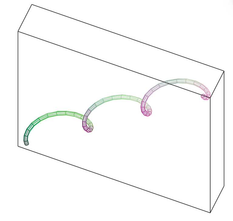
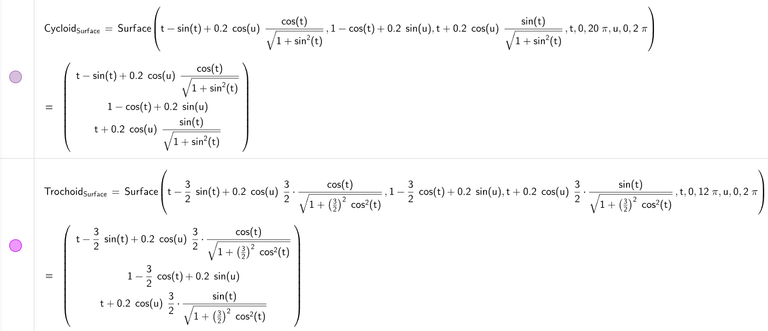
Here are the graphs in GeoGebra: https://www.geogebra.org/calculator/rmhpa57e

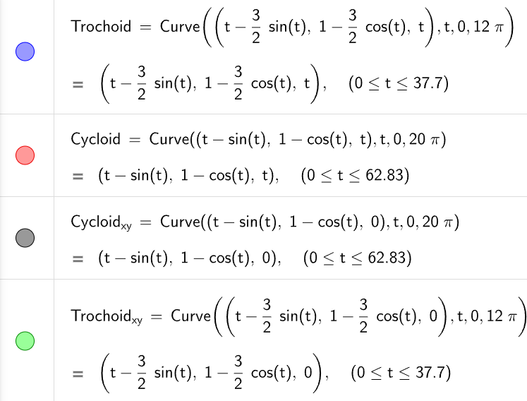
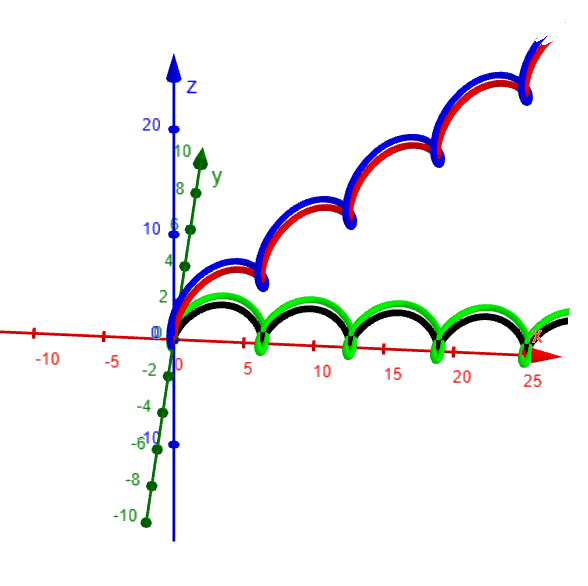
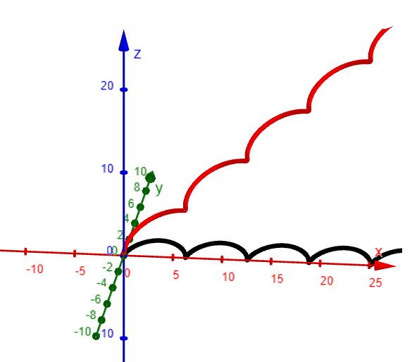
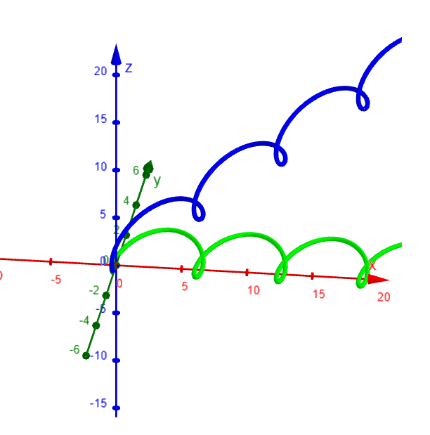
Since there is no Tube command in GeoGebra, I used the Surface command (via Grok AI) to generate a circular cross section of the curves.

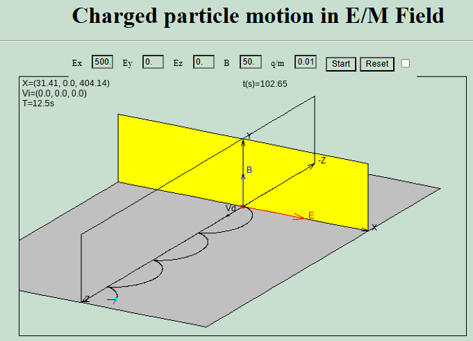
The Physics of Charged Particles in Electromagnetic Fields

For further details concerning the physics involved and animations of the trajectories of particles, see the following websites:

• https://www.phy.ntnu.edu.tw/java/emField/emField.html
  • Note that to run this website, you'll need to run Java Applets, which you can with this Browser extension: https://cheerpj.com/cheerpj-applet-runner/
• https://www.physics.ucla.edu/plasma-exp/Beam/

Here is a quick review of those websites and more.

https://www.phy.ntnu.edu.tw/java/emField/emField.html

https://www.physics.ucla.edu/plasma-exp/Beam/

Single Particle Motion in Electric and Magnetic Fields

The following photographs were made in the Physics 180E undergraduate laboratory course in plasma physics by Professor Reiner L. Stenzel. They are designed to demonstrate the single particle motion in electric and magnetic fields. A weak electron beam of typically 100 eV, 1-10 mA is injected from an oxide-coated cathode into a low pressure (0.2 mTorr) argon gas. The beam partially ionizes the gas. The background plasma has a potential close to that of the grounded chamber wall. The beam electrons are accelerated by an electric field mainly concentrated in the cathode sheath. The trajectory of the beam electrons is visible due to light excitation when the beam electrons collide with argon atoms. No visible light is produced when the electron energy is below typically 10 eV. Several basic phenomena can be inferred from the following pictures. These were taken with a Rolleiflex camera, 400 ASA, black and white film, with up to one minute exposure time.

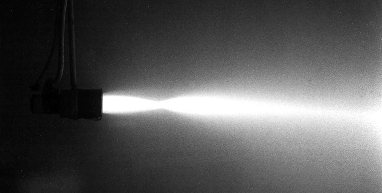
Fig. 1. A 100 eV electron beam is injected into a neutral gas without applying external electric or magnetic fields. The beam light starts very close to the cathode indicating that the electrons acquire their full energy in a very thin cathode sheath. Thus, the self-produced plasma acts as an anode. The initial beam convergence indicates concave equipotential surfaces near the cathode, presumably due to a radial density gradient. The beam scatters by collisions and beam-plasma instabilities.

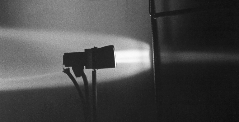
Fig. 2 The beam is injected against a negatively biased grid. When the bias voltage is slightly larger than the cathode voltage most of the beam is reflected but a few electrons are transmitted. Note that the equipotential surface near the grid is not plane but convex. This causes an angular spread of the reflected electrons. Electrons in the center of the beam are normal to the sheath and can pass the grid when their energy exceeds the potential energy of the sheath.

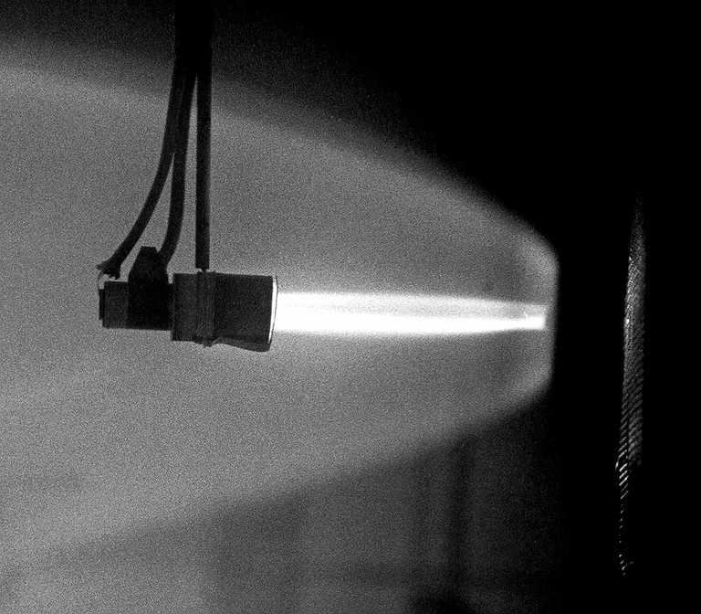
Fig. 3. Beam injection against a very negatively biased grid which reflects all electrons. Note dark sheath near grid where the electron energy is decreased below 10 eV. The electrons stagnate in the dark sheath and form a convex equipotential surface. This causes the reflected beam to be highly divergent.

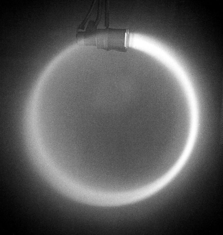
Fig. 4. A 100 eV electron beam injected perpendicular to a dc magnetic field. The sense of the cyclotron orbit implies that the magnetic field points into the plane. From the beam energy and the cyclotron radius the field strength can be calculated. Note that the beam light weakens with propagation distance

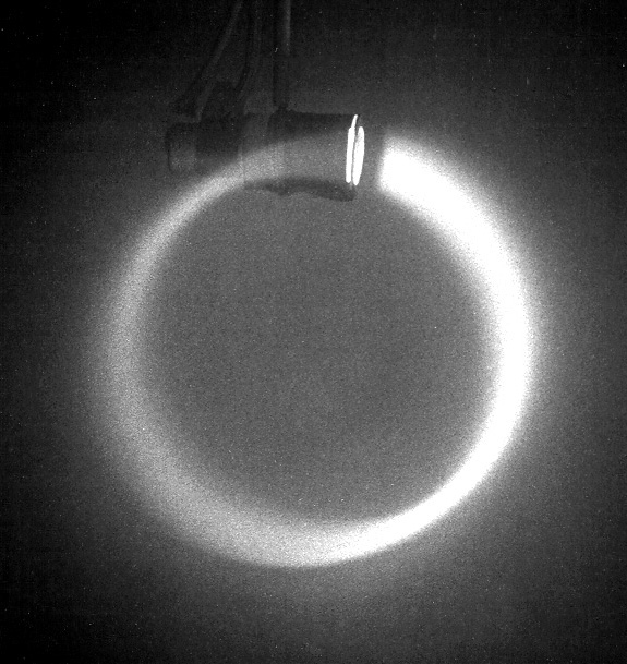
Fig. 5. A low energy beam is injected across a magnetic field as in Fig. 1 [Fig. 4?]. The cyclotron radius is decreased. Note the dark gap between the cathode and beam onset. In this sheath region the electrons still have insufficient energy for light excitation.

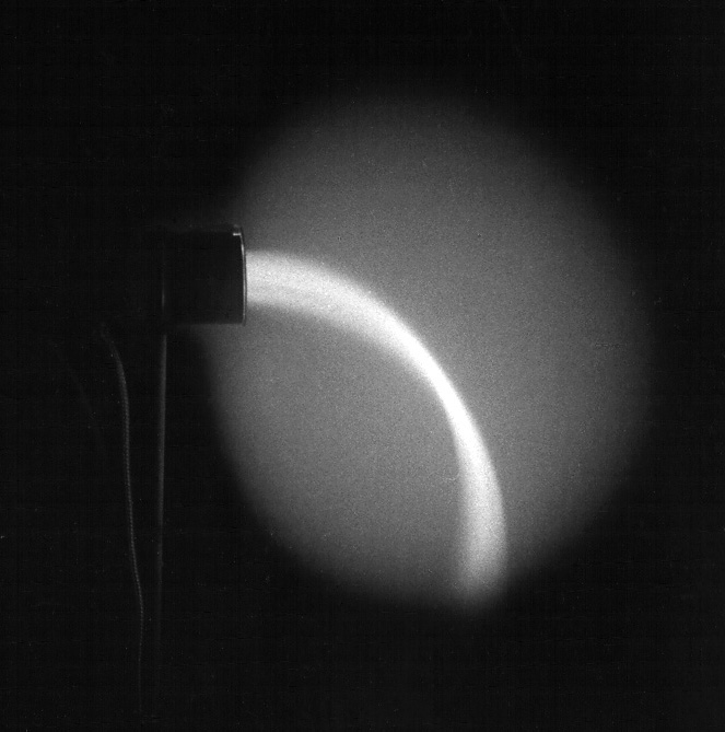
Fig. 6. A low energy beam is injected against a decelerating electric field. As the beam energy falls below 10 eV the light emission stops. The beam and current continue to flow through the dark region.

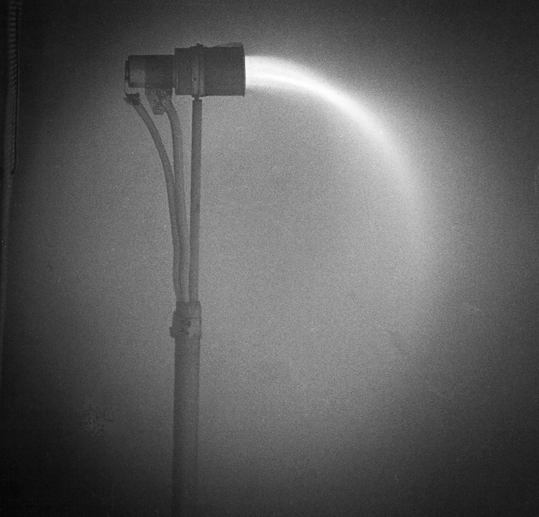
Fig. 7. At high neutral pressures the injected electron beam rapidly spreads. The electron mean free path can be inferred from the beam decay.

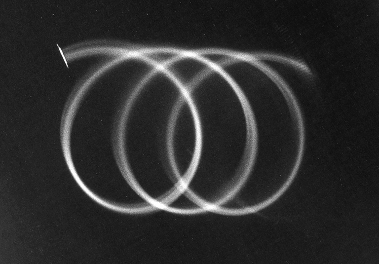
Fig. 8. Electron motion in crossed electric and magnetic fields. The trajectory is a cycloid [Trochoid], i.e., a superposition of a circular motion and a constant drift to the right. The cyclotron orbit implies a magnetic field direction into the plane and the E×B drift implies that the electric field points downward. From the known beam energy the field strengths can be obtained from cyclotron radius and guiding center drift.

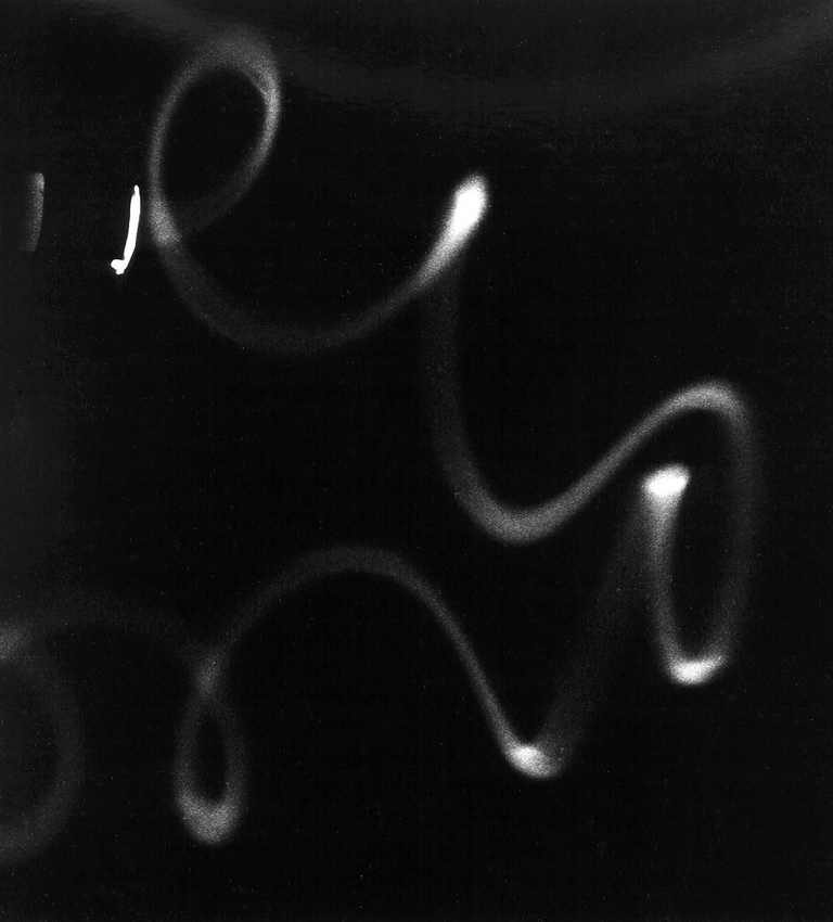
Fig. 9. Mirror reflection of a weak electron beam in a nonuniform magnetic field. The beam is injected oblique to the field lines which converge to the right. Due to the adiabatic invariants (energy and magnetic moment) the parallel energy is converted into perpendicular energy at which point the particles reflect. Alternatively, the parallel motion is decelerated by the repelling force of an increasing magnetic field.

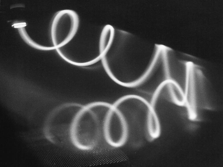
Fig. 10. Mirror reflection of a stronger electron beam in a magnetic field which converges to the right. Note that the guiding center (axis of spiral) of the reflected beam does not coincide with that of the incident. This is due to the gradient and curvature drift in a nonuniform field.

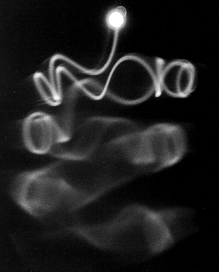
Fig 11. Multiple reflections of an oblique electron beam in a mirror magnetic field. The cyclotron motion is the fastest periodic motion, followed by the slower bounce motion between the mirror points. Gradient and curvature drifts cause a third, slowest rotation azimuthally around the mirror axis. This is the classical charged particle motion in the ionosphere in Earth's magnetic dipole field. Collisions and other scattering processes diffuse the beam.

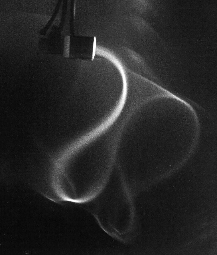
Fig.12. Electron beam injected into a nonuniform magnetic field with a null line. The beam meanders along a magnetic null line pointing diagonally down to the right. Note the reversal of the cyclotron rotation as the magnetic field reverses to either side of the neutral line. Such meandering and figure-eight trajectories have been studied theoretically in the problem of magnetic reconnection occurring in the magnetosphere and on the sun.

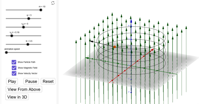
Here is an amazing Charged Particle in a Magnetic Field 3D calculator Tom Walsh made in GeoGebra: https://www.geogebra.org/m/qajRP2O4

Note that the charged particle is plotted with all axes in space, and none in time as with the cycloid / trochoid graphs.

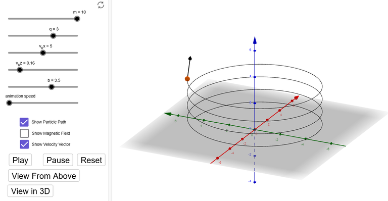
Note that a moving charged particle experiences a Lorentz force from a magnetic field according to the right hand rule:

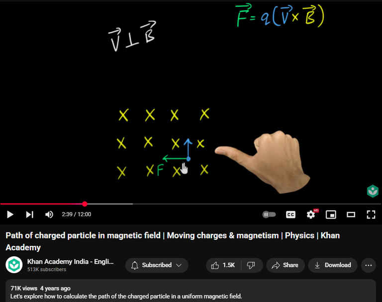
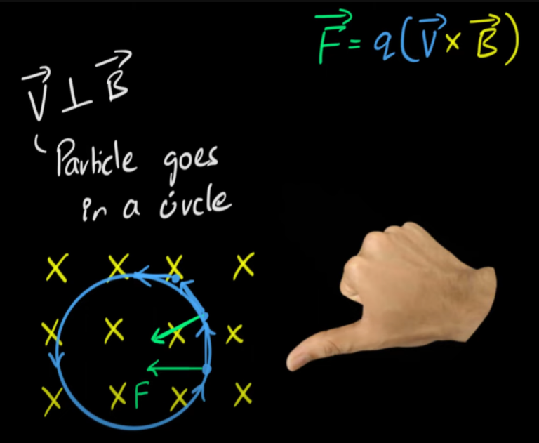
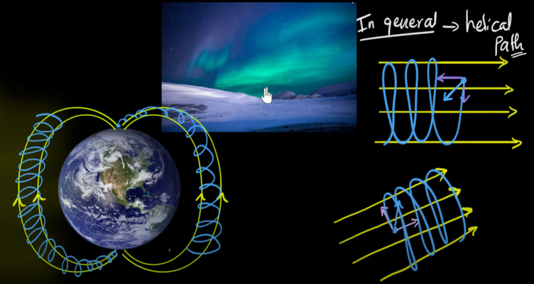
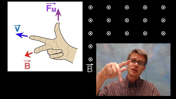
Right hand rule video.

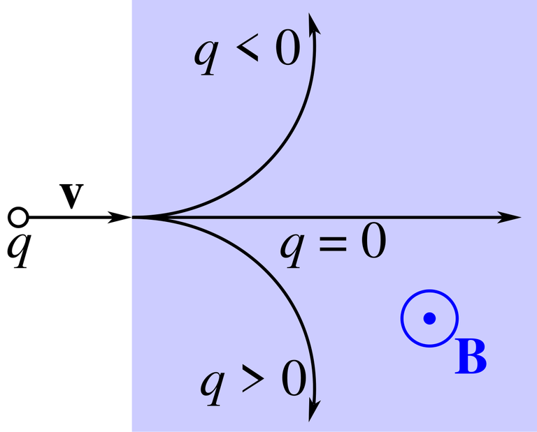
Trajectory of a particle with a positive or negative charge q under the influence of a magnetic field B, which is directed perpendicularly out of the screen

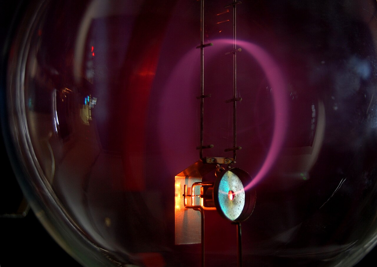
Beam of electrons moving in a circle, due to the presence of a magnetic field. Purple light revealing the electron's path in this Teltron tube is created by the electrons colliding with gas molecules.

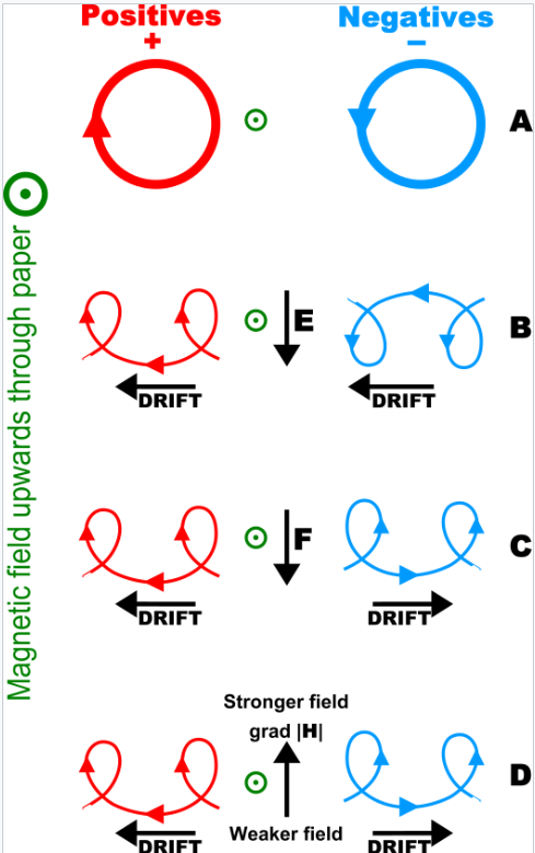
Charged particle drifts in a homogeneous magnetic field. (A) No disturbing force. (B) With an electric field, E. (C) With an independent force, F (e.g. gravity). (D) In an inhomogeneous magnetic field, grad H.

MES Note: Is gravity just a magnetic field gradient?!

---

Exercises

---

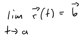
Exercise 1: Precise Definition of a Vector Function Limit

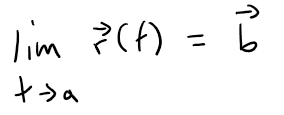
Show that:

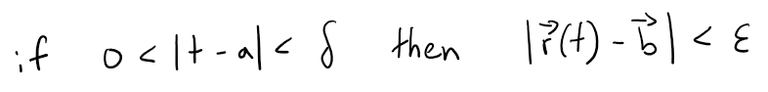
if and only if for every ε > 0 there is a number δ > 0 such that:

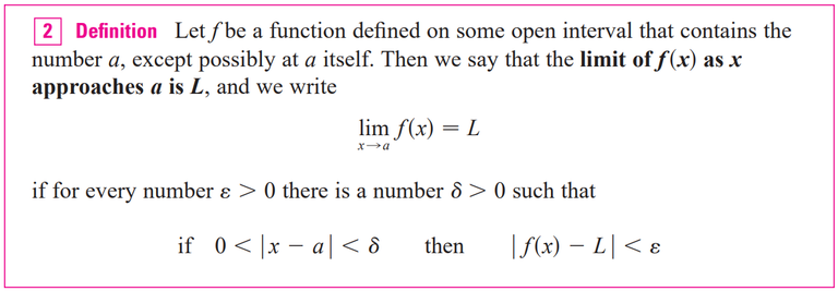
Recap on Limits:

Recall the precise definition of a real-valued function from my earlier video:

Solution 1

Let r(t) be a vector defined on some open interval containing t = a, except possibly at a itself.

Let b be a vector in R³.

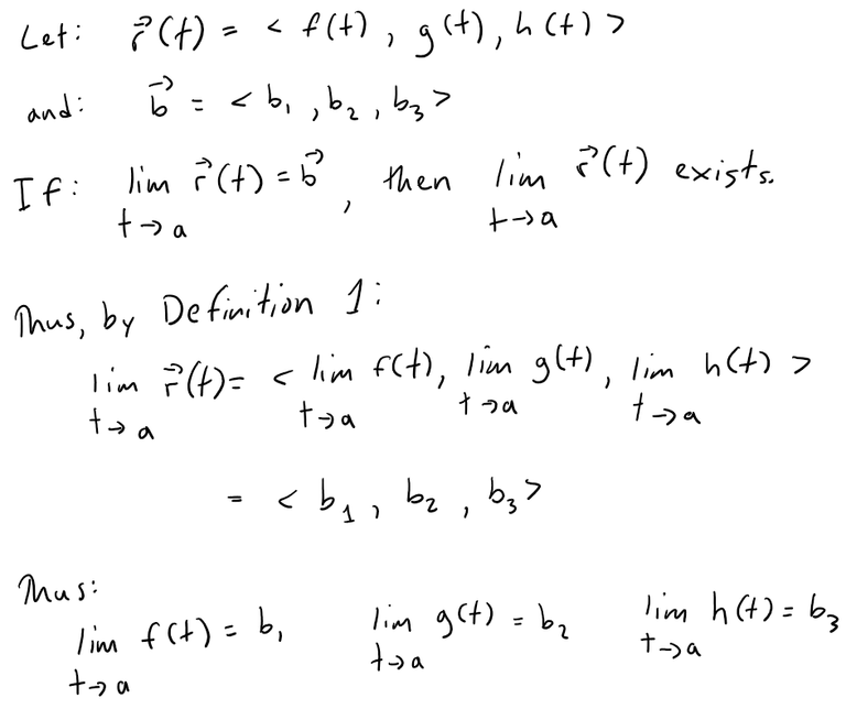
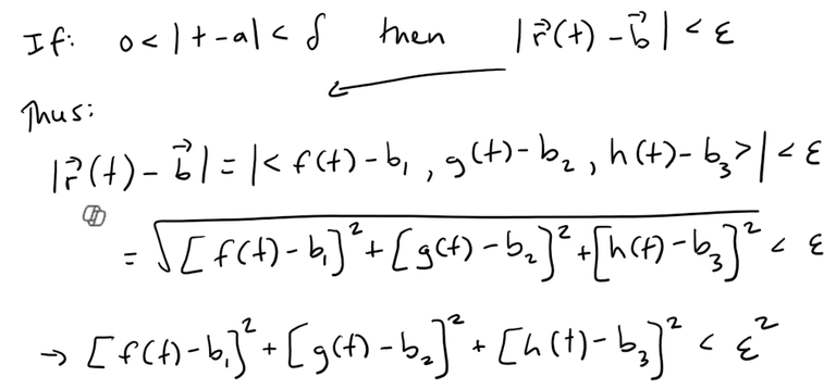
But these are limits of real-valued functions, so by the definition of limits, for every ε > 0 there exists δ₁ > 0, δ₂ > 0, and δ₃ > 0 such that:

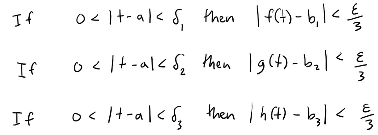
Letting δ = minimum of {δ₁ > 0, δ₂ > 0, δ₃}, then:

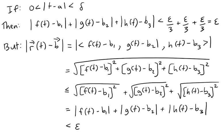
Thus for every ε > 0 there exists δ > 0 such that:

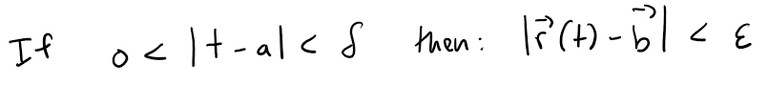
This proves our limit.

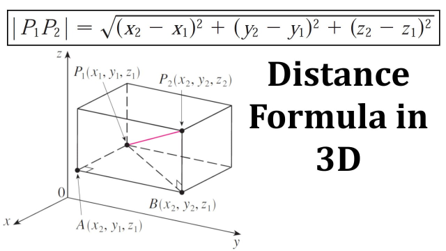
Note that I used the distance formula in 3D from my earlier video:

Solution 2

Conversely, suppose for every ε > 0, there exists δ > 0 such that:

But each term on the left side of the above inequality is positive, thus:

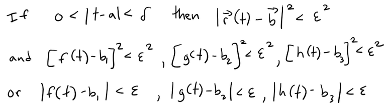
And by definition of limits of real-valued functions, we have:

But by Definition 1, we have:

Visualizing the Precise Definition of a Vector Function Limit

We can visualize the definition in 3D in just the same way as we did in 2D.

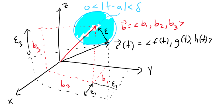
This means that as we shrink the interval of the parameter t (by picking a smaller δ) then the difference between r and b get smaller (ε gets smaller), and we can keep doing this indefinitely.

---

Exercise 2: Properties of Vector Function Limits

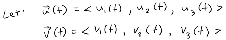
Suppose u and v are vector functions that possess limits as t → a and let c be a constant.

Prove the following properties:

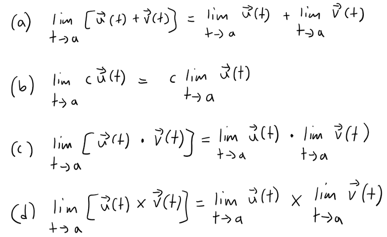
Solution:

In each part of this problem, the basic procedure is to use Definition 1 and then analyze the individual component functions using the limit properties we have already developed for real-valued functions.

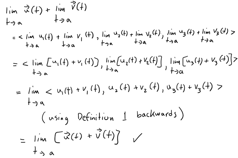
Solution to (a)

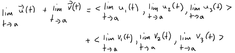
The limits of these component functions must each exist since the vector functions both possess limits as t → a (i.e. if the limits of the vector functions exist, then so does their component functions).

Then adding the two vectors and using the addition property of limits for real-valued functions, we have that:

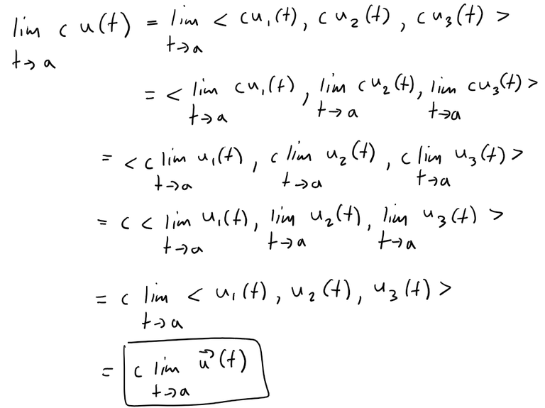
Solution to (b)

Solution to (c)

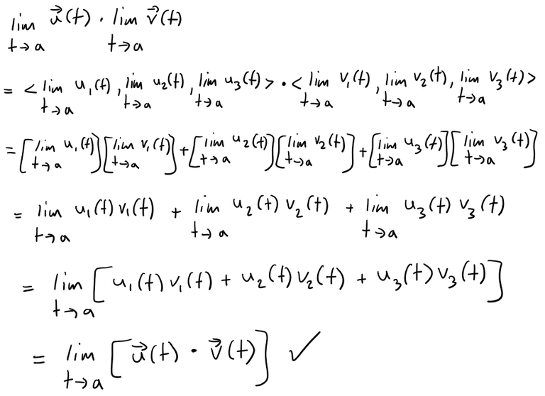
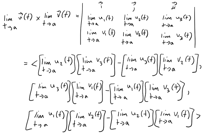
Solution to (d)

---

Exercise 3: Trefoil Knot

The view of the trefoil knot shown earlier (and copied below) is accurate but it doesn't reveal the whole story.

x = (2 + cos 1.5t) cos t
y = (2 + cos 1.5t) sin t
z = sin 1.5t

A trefoil knot

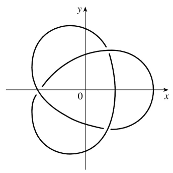
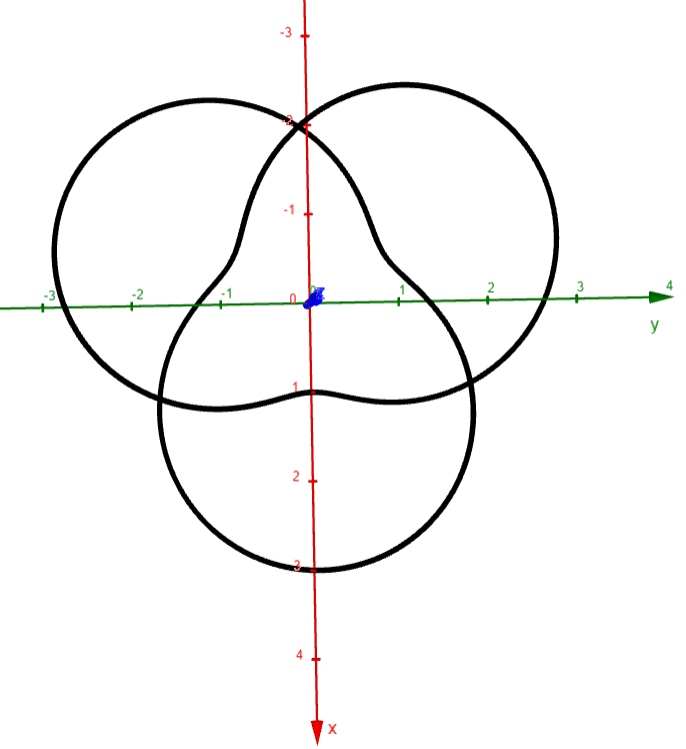
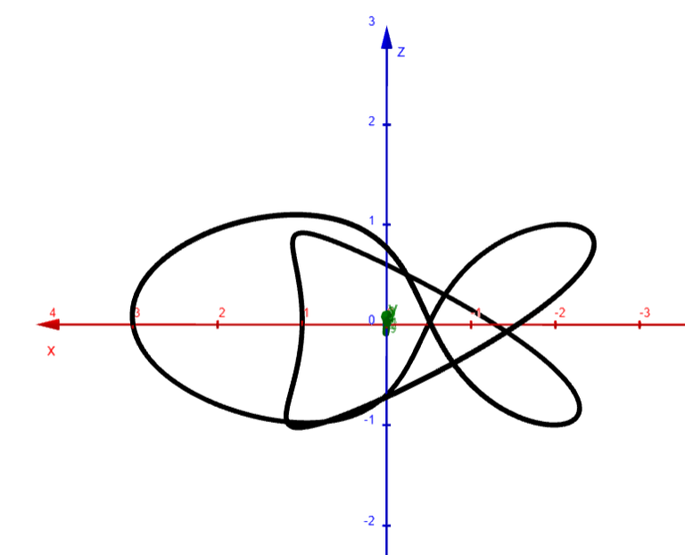
Use the following parametric equations to sketch the curve by hand as viewed from above, with gaps indicating where the curve passes over itself.

x = (2 + cos 1.5t) cos t
y = (2 + cos 1.5t) sin t
z = sin 1.5t

Start by showing that the projection of the curve onto the xy-plane has polar coordinates r = 2 + cos 1.5t and θ = t, so r varies between 1 and 3.

Then show that z has maximum and minimum values when the projection is halfway between r = 1 and r = 3.

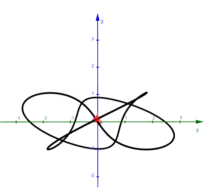
When you have finished your sketch, use a computer to draw the curve with viewpoint directly above and compare with your sketch.

Then use the computer to draw the curve from several other viewpoints.

You can get a better impression of the curve if you plot a tube with radius 0.2 around the curve.

Use the tubeplot command in Maple or the tubecurve or Tube command in Mathematica.

Solution:

The projection of the curve onto the xy-plane is given by the parametric equations:

x = (2 + cos 1.5t) cos t
y = (2 + cos 1.5t) sin t
z = 0

We can convert to polar coordinates by finding the distance r from the origin:

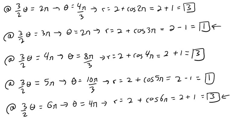
At θ = 0, we have r = 3, and r decreases to 1 as θ increases to 2π/3.

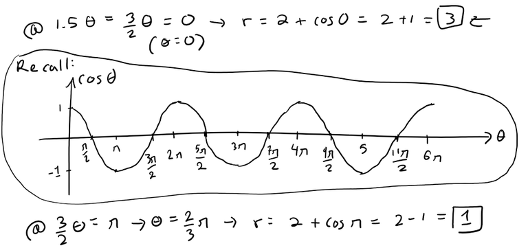
For 2π/3 ≤ θ ≤ 4π/3, r increases to 3; r decreases to 1 again at θ = 2π, increases to 3 at θ = 8π/3, decreases to 1 at θ = 10π/3, and completes the closed curve by increasing to 3 at θ = 4π.

We sketch an approximate graph as shown in the figure below.

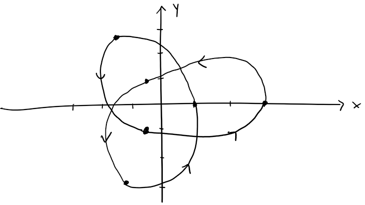
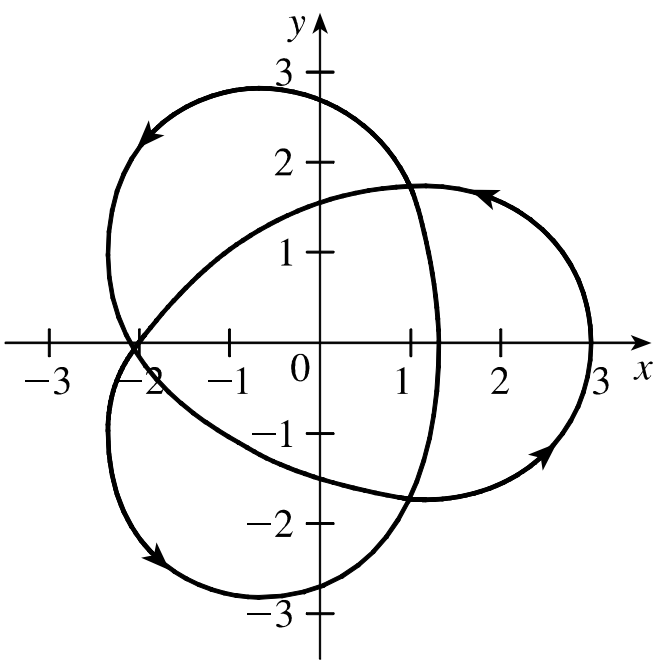
Here is a better sketch from the Solution Manual.

We can determine how the curve passes over itself by investigating the maximum and minimum values for z for 0 ≤ t ≤ 4π.

Since z = sin 1.5t, z is maximized where sin 1.5t = 1, thus:

z is minimized where sin 1.5t = -1, thus:

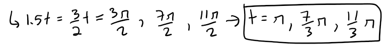
Note that these are precisely the values (both the minimum and maximum) for which cos 1.5t = 0:

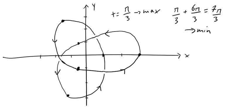
On the graph of the projection, these six points appear to be at the three self-intersections we see.

Comparing the maximum and minimum values of z at these intersections we can determine where the curve passes over itself, as indicated in the figure below.

Here is a better sketch from my Calculus book solution manual:

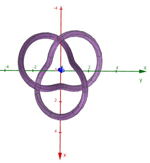
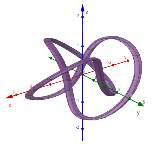
We show a computer-drawn graph of the curve from above, as well as views from the front and from the right side.

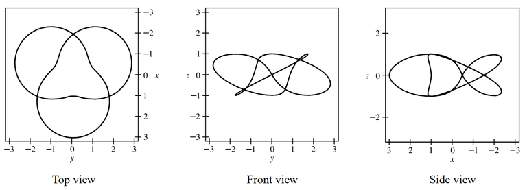
The top view graph shows a more accurate representation of the projection of the trefoil knot onto the xy-plane (the axes are rotated 90°).

Notice the indentations the graph exhibits at the points corresponding to r = 1.

Finally, we graph several additional viewpoints of the trefoil knot, along with two plots showing a tube of radius 0.2 around the curve.

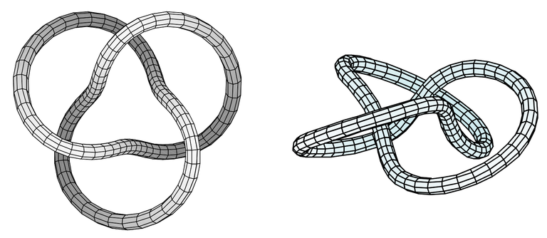
Here is the trefoil knot plotted in GeoGebra: https://www.geogebra.org/calculator/ckmexx42

Note that GeoGebra doesn't have a Tube command, so I had to create a surface (via Grok AI) that has a circular cross section around the Trefoil Knot curve.

Here is the same plot in Desmos' new 3D Graphing calculator: https://www.desmos.com/3d/dn5bonsvwf

---

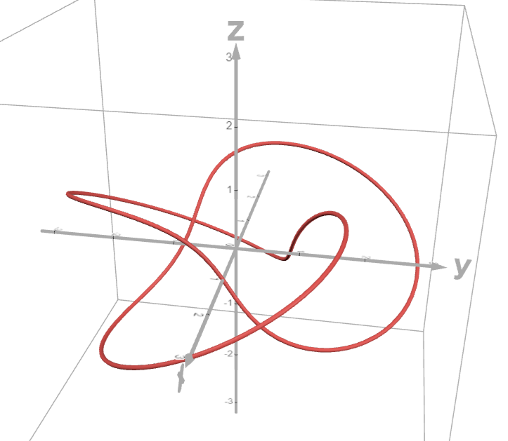
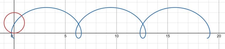
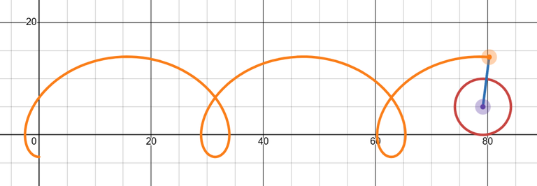
Exercise 4: The Trochoid

Note: This exercise is from an earlier chapter on Parametric Equations and Polar Coordinates, but I had not done a video on this particular exercise.

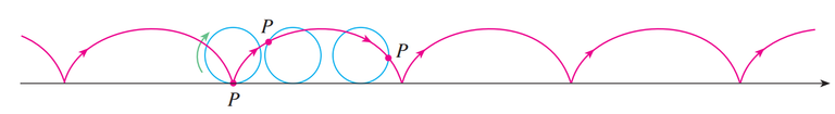
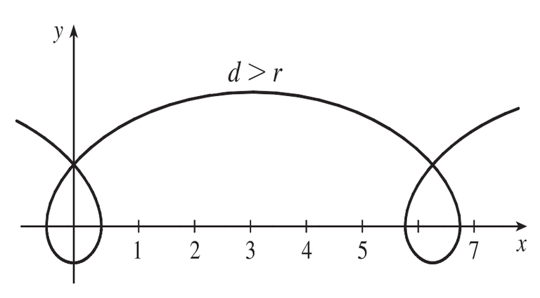
Let P be a point at a distance d from the center of a circle of radius r.

The curve traced out by P as the circle rolls along a straight line is called a trochoid.

Think of the motion of a point on a spoke of a bicycle wheel.

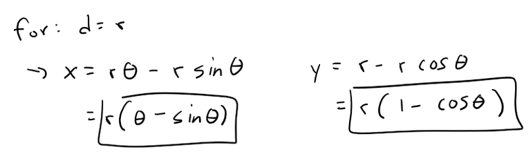
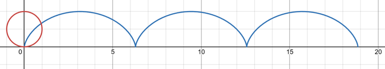
The cycloid is the special case of a trochoid with d = r.

The trochoid is formed by tracing any point inside, on (hence a cycloid), or outside a circle as it rolls.

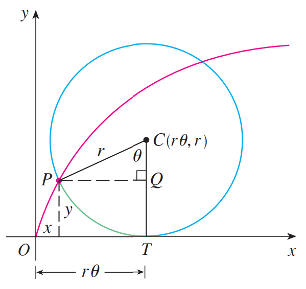
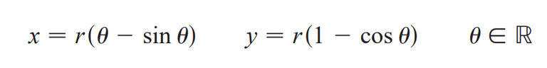
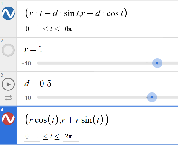
Using the same parameter θ as for the cycloid and, assuming the line is the x-axis and θ = 0 when P is at one of its lowest points, show that parametric equations of the trochoid are:

x = r θ - d sin θ
y = r - d cos θ

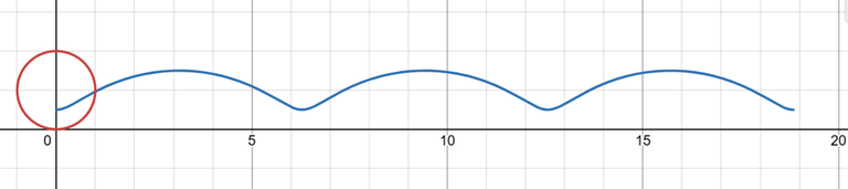
Sketch the trochoid for the cases d < r and d > r.

Solution:

Recall from my earlier video on the cycloid.

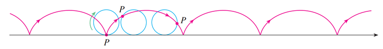
The first two diagrams below depict a curtate trochoid (d < r) for π < θ < 3π/2:

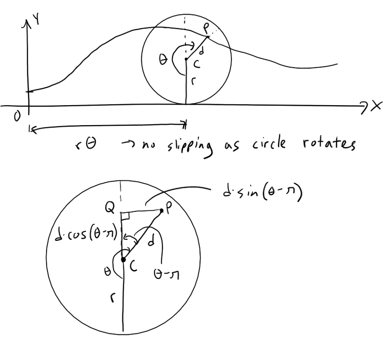
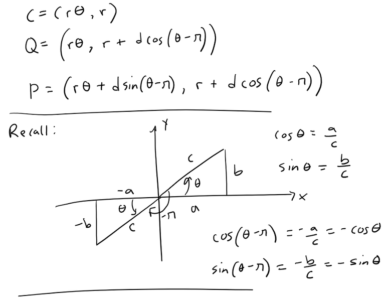
As for the cycloid, the center C of the circle has coordinates (rθ, r) since there is no slipping as the circle rotates (the distance traveled is just the arc length that has rolled on the ground).

The coordinates of Q and P are thus:

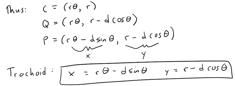
When d = r, these parametric equations of a trochoid agree with those of a cycloid.

A prolate trochoid (d > r) is graphed below:

Here are graphs of the trochoid using the Desmos 2D graphing calculator. https://www.desmos.com/calculator/zrw9kc2tmb

And here is an amazing Trochoid animator someone made on Desmos: https://www.desmos.com/calculator/1orvf2yhrk

#EpicStuff!